
AI in Stock Market
The most fundamental motivation for trying to predict the stock market prices is financial gain. The ability to uncover a precise model that can predict the path of the future stock prices would make the owner of the method extremely wealthy. Investors and investment firms are always searching to find a stock market model that would give them the best return on investment at the time.
This project will cover the TESLA stock and I will be doing analysis against it. I have used three different methods in attempt to get the best result at guessing the open price of the next day. There is a huge market for being able to try and predict the price of stock. Many different companies are specializing and investing huge amounts of money into trying to do this action.
From what I have found it is not possible to simply estimate what the stock will be weeks or months ahead. So for this project I have taken the timeline of just a day. A day might be able to be feasible in this project and will produce trackable results.
from alpha_vantage.timeseries import TimeSeries
import pandas as pd
import matplotlib.pyplot as plt
import numpy as np

alpha_vantage_api_key = "XXXX"
def pull_daily_time_series_alpha_vantage(alpha_vantage_api_key, ticker_name, output_size = "full"):
    ts = TimeSeries(key = alpha_vantage_api_key, output_format = 'pandas')
    data, meta_data = ts.get_daily_adjusted(ticker_name, outputsize = output_size)
    data['date_time'] = data.index
    return data, meta_data
Data
The Alpha Vatange API allows me to call in all the historical data from TESLA so that I have the necessary data to perform analysis. I have three main variables that I am looking at which are; volume, open, close, high, and low. Since I am only running this off a MacBook Air I want to make sure that my data is able to run at in resonible timeframe so I decided to limit the amount of variables that I am using.
def plot_data(df, x_variable, y_variable, title):
    fig, ax = plt.subplots()
    ax.plot_date(df[x_variable],
                 df[y_variable], marker='', linestyle='-', label=y_variable)
    fig.autofmt_xdate()
    plt.title(title)
    plt.show()
ts_data, ts_metadata = pull_daily_time_series_alpha_vantage(alpha_vantage_api_key, ticker_name = "TSLA", output_size = "full")
plot_data(df = ts_data,
          x_variable = "date_time",
          y_variable = "1. open",
          title ="Open Values, Tesla Stock, Daily Data")
/Users/lukegruszka/anaconda3/lib/python3.7/site-packages/pandas/plotting/_converter.py:129: FutureWarning: Using an implicitly registered datetime converter for a matplotlib plotting method. The converter was registered by pandas on import. Future versions of pandas will require you to explicitly register matplotlib converters.

To register the converters:
	>>> from pandas.plotting import register_matplotlib_converters
	>>> register_matplotlib_converters()
  warnings.warn(msg, FutureWarning)

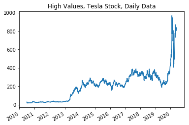
plot_data(df = ts_data,
          x_variable = "date_time",
          y_variable = "2. high",
          title ="High Values, Tesla Stock, Daily Data")
plot_data(df = ts_data,
          x_variable = "date_time",
          y_variable = "3. low",
          title ="Low Values, Tesla Stock, Daily Data")

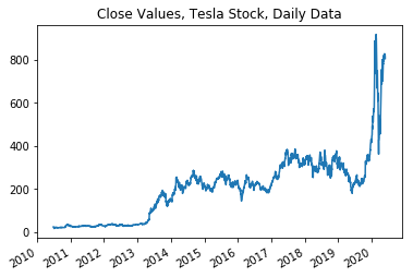
plot_data(df = ts_data,
          x_variable = "date_time",
          y_variable = "4. close",
          title ="Close Values, Tesla Stock, Daily Data")
plot_data(df = ts_data,
          x_variable = "date_time",
          y_variable = "6. volume",
          title ="Volume, Tesla Stock, Daily Data")
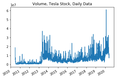
Here I am investigating how the variables graph against time. As we can see from the graphs and then the correlations below; there are many correlations between the variables that are worth investigating before determining the algorithms and functions that I will be using below.
high_low_corr = np.corrcoef(x = ts_data["2. high"],
                            y = ts_data["3. low"])
high_low_corr
array([[1.        , 0.99882357],
       [0.99882357, 1.        ]])
high_close_corr = np.corrcoef(x = ts_data["2. high"],
                            y = ts_data["4. close"])
high_close_corr
array([[1.       , 0.9993323],
       [0.9993323, 1.       ]])
low_close_corr = np.corrcoef(x = ts_data["4. close"],
                            y = ts_data["3. low"])
low_close_corr
array([[1.        , 0.99937197],
       [0.99937197, 1.        ]])
volume_close_corr = np.corrcoef(x = ts_data["4. close"],
                            y = ts_data["6. volume"])
volume_close_corr
array([[1.        , 0.58532154],
       [0.58532154, 1.        ]])
open_close_corr = np.corrcoef(x = ts_data["4. close"],
                            y = ts_data["1. open"])
open_close_corr
array([[1.        , 0.99870754],
       [0.99870754, 1.        ]])
ts_data.describe()
| 1. open | 2. high | 3. low | 4. close | 5. adjusted close | 6. volume | 7. dividend amount | 8. split coefficient | |
|---|---|---|---|---|---|---|---|---|
| count | 2496.000000 | 2496.000000 | 2496.000000 | 2496.000000 | 2496.000000 | 2.496000e+03 | 2496.0 | 2496.0 |
| mean | 202.734893 | 206.663082 | 198.661582 | 202.769225 | 202.769225 | 5.985255e+06 | 0.0 | 1.0 |
| std | 149.788794 | 153.480925 | 145.954729 | 149.761358 | 149.761358 | 5.625749e+06 | 0.0 | 0.0 |
| min | 16.140000 | 16.630000 | 14.980000 | 15.800000 | 15.800000 | 1.185000e+05 | 0.0 | 1.0 |
| 25% | 34.930000 | 35.432500 | 34.325500 | 34.922500 | 34.922500 | 1.985670e+06 | 0.0 | 1.0 |
| 50% | 216.710000 | 220.525000 | 212.525000 | 216.980000 | 216.980000 | 4.704271e+06 | 0.0 | 1.0 |
| 75% | 279.140000 | 284.722500 | 275.297500 | 279.900000 | 279.900000 | 7.736158e+06 | 0.0 | 1.0 |
| max | 923.500000 | 968.989900 | 901.020000 | 917.420000 | 917.420000 | 6.093876e+07 | 0.0 | 1.0 |
As we can see from the data describe above that the variables show extreme relevance towards each other except for the volume. The Volume seems to be the odd variable out that doesn’t follow the trends of the other variables.
MODEL LINEAR AND VECTOR
Support Vector Regression (SVR)
This is a supervised learning algorithm that analyzes data for regression analysis. It is effective in high dimensional spaces, works will with a clear margin or separation and it is great when the dimensions are greater than the number of samples that you are providing.
One issue that I am anticipating is that it does not perform well with a large data set. I am using a lot of data to run analysis and I fear that this algorithm will not perform up to the standard.
Linear Regression
This is a linear approach to showing a relationship between a dependent variable and independent variables. This is very easy to create and run and it is a great way to predict numerical values.
from sklearn.linear_model import LinearRegression
from sklearn.svm import SVR
from sklearn.model_selection import train_test_split
df = ts_data[['4. close']]
df.head()
| 4. close | |
|---|---|
| date | |
| 2010-06-29 | 23.89 |
| 2010-06-30 | 23.83 |
| 2010-07-01 | 21.96 |
| 2010-07-02 | 19.20 |
| 2010-07-06 | 16.11 |
I will be predicting the value for one day out into the furture. I will be focusing on the closing value to try and predict weather or not we can be confidence that the value will go up in the future or is the value will decrease in the future.
forecast_out = 1
df['Prediction'] = df[['4. close']].shift(-forecast_out)
print(df.tail())
            4. close  Prediction
date
2020-05-21    827.60      816.88
2020-05-22    816.88      818.87
2020-05-26    818.87      820.23
2020-05-27    820.23      805.81
2020-05-28    805.81         NaN


/Users/lukegruszka/anaconda3/lib/python3.7/site-packages/ipykernel_launcher.py:4: SettingWithCopyWarning:
A value is trying to be set on a copy of a slice from a DataFrame.
Try using .loc[row_indexer,col_indexer] = value instead

See the caveats in the documentation: http://pandas.pydata.org/pandas-docs/stable/indexing.html#indexing-view-versus-copy
  after removing the cwd from sys.path.
X = np.array(df.drop(['Prediction'],1))
X = X[:-forecast_out]
print(X)
[[ 23.89]
 [ 23.83]
 [ 21.96]
 ...
 [816.88]
 [818.87]
 [820.23]]
y = np.array(df['Prediction'])
y = y[:-forecast_out]
print(y)
[ 23.83 21.96 19.2 ... 818.87 820.23 805.81]
In order to be able to run the algorithms I will need to split my data into a 80 / 20 split that I will use for the training and testing data. I will Create and train the Support Vector Machine (Regressor) and Linear Regression. When testing the model, the score returns the coefficient of determination R^2 of the prediction. The best possible score is 1.0
x_train, x_test, y_train, y_test = train_test_split(X, y, test_size=0.2)
svr_rbf = SVR(kernel='rbf', C=1e3, gamma=0.1)
svr_rbf.fit(x_train, y_train)
SVR(C=1000.0, cache_size=200, coef0=0.0, degree=3, epsilon=0.1, gamma=0.1,
  kernel='rbf', max_iter=-1, shrinking=True, tol=0.001, verbose=False)
svm_confidence = svr_rbf.score(x_test, y_test)
print("svm confidence: ", svm_confidence)
svm confidence: 0.9461082109077223
lr = LinearRegression()
lr.fit(x_train, y_train)
LinearRegression(copy_X=True, fit_intercept=True, n_jobs=None,
         normalize=False)
lr_confidence = lr.score(x_test, y_test)
print("lr confidence: ", lr_confidence)
lr confidence: 0.9917606082822382
Set x_forecast equal to the last 30 rows of the original data set from Adj. Close column
x_forecast = np.array(df.drop(['Prediction'],1))[-forecast_out:]
print(x_forecast)
[[805.81]]
lr_prediction = lr.predict(x_forecast)
print(lr_prediction)
print()
svm_prediction = svr_rbf.predict(x_forecast)
print(svm_prediction)
[807.74776292]

[737.05526653]
MODEL NEURAL NETWORK
From what I can see above I can see that the numbers are very different. Unless something goes horribly wrong I can not agree with the SVM result of 737. However, I was pleased with the Linear Regression model that produced 807. But now I wanted to run this data against a Neural Network. The setup should be the same with finding the 80 / 20 split but will require some reshaping to make sure that my data will fit into the layers that I want.
from sklearn.preprocessing import MinMaxScaler
from keras.models import Sequential, load_model
from keras.layers import LSTM, Dense, Dropout
import os
dfNN = ts_data[['1. open','2. high','3. low','4. close']]
dfNN.tail()
Using TensorFlow backend.
| 1. open | 2. high | 3. low | 4. close | |
|---|---|---|---|---|
| date | ||||
| 2020-05-21 | 816.0000 | 832.50 | 796.000 | 827.60 |
| 2020-05-22 | 822.1735 | 831.78 | 812.000 | 816.88 |
| 2020-05-26 | 834.5000 | 834.60 | 815.705 | 818.87 |
| 2020-05-27 | 820.8600 | 827.71 | 785.000 | 820.23 |
| 2020-05-28 | 813.5100 | 824.75 | 801.690 | 805.81 |
dfClose = dfNN['4. close'].values
dfClose = dfClose.reshape(-1,1)
dfClose
array([[ 23.89],
       [ 23.83],
       [ 21.96],
       ...,
       [818.87],
       [820.23],
       [805.81]])
dataset_train = np.array(dfClose[:int(dfClose.shape[0]*0.8)])
dataset_test = np.array(dfClose[int(dfClose.shape[0]*0.8)-50:])
print(dataset_train.shape)
print(dataset_test.shape)
(1996, 1)
(550, 1)
scaler = MinMaxScaler(feature_range=(0,1))
dataset_train = scaler.fit_transform(dataset_train)
dataset_test = scaler.transform(dataset_test)
def create_dataset(dfClose):
    xClose = []
    yClose = []
    for i in range(50, dfClose.shape[0]):
        xClose.append(dfClose[i-50:i, 0])
        yClose.append(dfClose[i, 0])
    xClose = np.array(xClose)
    yClose = np.array(yClose)
    return xClose,yClose
x_train, y_train = create_dataset(dataset_train)
x_test, y_test = create_dataset(dataset_test)
x_train = np.reshape(x_train, (x_train.shape[0], x_train.shape[1], 1))
x_test = np.reshape(x_test, (x_test.shape[0], x_test.shape[1], 1))
model = Sequential()
model.add(LSTM(units=96, return_sequences=True, input_shape=(x_train.shape[1], 1)))
model.add(Dropout(0.2))
model.add(LSTM(units=96, return_sequences=True))
model.add(Dropout(0.2))
model.add(LSTM(units=96, return_sequences=True))
model.add(Dropout(0.2))
model.add(LSTM(units=96))
model.add(Dropout(0.2))
model.add(Dense(units=1))
WARNING:tensorflow:From /Users/lukegruszka/anaconda3/lib/python3.7/site-packages/tensorflow/python/ops/resource_variable_ops.py:435: colocate_with (from tensorflow.python.framework.ops) is deprecated and will be removed in a future version.
Instructions for updating:
Colocations handled automatically by placer.
model.compile(loss='mean_squared_error', optimizer='adam')
model.fit(x_train, y_train, epochs=50, batch_size=32)
model.save('stock_prediction.h5')
model = load_model('stock_prediction.h5')
WARNING:tensorflow:From /Users/lukegruszka/anaconda3/lib/python3.7/site-packages/tensorflow/python/ops/math_ops.py:3066: to_int32 (from tensorflow.python.ops.math_ops) is deprecated and will be removed in a future version.
Instructions for updating:
Use tf.cast instead.
Epoch 1/50
1946/1946 [==============================] - 14s 7ms/step - loss: 0.0158
Epoch 2/50
1946/1946 [==============================] - 10s 5ms/step - loss: 0.0035
Epoch 3/50
1946/1946 [==============================] - 10s 5ms/step - loss: 0.0036
Epoch 4/50
1946/1946 [==============================] - 10s 5ms/step - loss: 0.0032
Epoch 5/50
1946/1946 [==============================] - 10s 5ms/step - loss: 0.0029
Epoch 6/50
1946/1946 [==============================] - 10s 5ms/step - loss: 0.0029
Epoch 7/50
1946/1946 [==============================] - 10s 5ms/step - loss: 0.0033
Epoch 8/50
1946/1946 [==============================] - 10s 5ms/step - loss: 0.0025
Epoch 9/50
1946/1946 [==============================] - 10s 5ms/step - loss: 0.0024
Epoch 10/50
1946/1946 [==============================] - 10s 5ms/step - loss: 0.0023
Epoch 11/50
1946/1946 [==============================] - 10s 5ms/step - loss: 0.0025
Epoch 12/50
1946/1946 [==============================] - 10s 5ms/step - loss: 0.0019
Epoch 13/50
1946/1946 [==============================] - 10s 5ms/step - loss: 0.0022
Epoch 14/50
1946/1946 [==============================] - 10s 5ms/step - loss: 0.0027
Epoch 15/50
1946/1946 [==============================] - 10s 5ms/step - loss: 0.0019
Epoch 16/50
1946/1946 [==============================] - 10s 5ms/step - loss: 0.0020
Epoch 17/50
1946/1946 [==============================] - 10s 5ms/step - loss: 0.0020
Epoch 18/50
1946/1946 [==============================] - 10s 5ms/step - loss: 0.0019
Epoch 19/50
1946/1946 [==============================] - 10s 5ms/step - loss: 0.0018
Epoch 20/50
1946/1946 [==============================] - 10s 5ms/step - loss: 0.0024
Epoch 21/50
1946/1946 [==============================] - 10s 5ms/step - loss: 0.0016
Epoch 22/50
1946/1946 [==============================] - 10s 5ms/step - loss: 0.0017
Epoch 23/50
1946/1946 [==============================] - 10s 5ms/step - loss: 0.0016
Epoch 24/50
1946/1946 [==============================] - 10s 5ms/step - loss: 0.0016
Epoch 25/50
1946/1946 [==============================] - 10s 5ms/step - loss: 0.0018
Epoch 26/50
1946/1946 [==============================] - 10s 5ms/step - loss: 0.0017
Epoch 27/50
1946/1946 [==============================] - 10s 5ms/step - loss: 0.0015
Epoch 28/50
1946/1946 [==============================] - 10s 5ms/step - loss: 0.0016
Epoch 29/50
1946/1946 [==============================] - 10s 5ms/step - loss: 0.0015
Epoch 30/50
1946/1946 [==============================] - 10s 5ms/step - loss: 0.0017
Epoch 31/50
1946/1946 [==============================] - 10s 5ms/step - loss: 0.0016
Epoch 32/50
1946/1946 [==============================] - 10s 5ms/step - loss: 0.0014
Epoch 33/50
1946/1946 [==============================] - 10s 5ms/step - loss: 0.0014
Epoch 34/50
1946/1946 [==============================] - 10s 5ms/step - loss: 0.0012
Epoch 35/50
1946/1946 [==============================] - 10s 5ms/step - loss: 0.0013
Epoch 36/50
1946/1946 [==============================] - 10s 5ms/step - loss: 0.0016
Epoch 37/50
1946/1946 [==============================] - 10s 5ms/step - loss: 0.0014
Epoch 38/50
1946/1946 [==============================] - 11s 5ms/step - loss: 0.0012
Epoch 39/50
1946/1946 [==============================] - 11s 6ms/step - loss: 0.0012
Epoch 40/50
1946/1946 [==============================] - 10s 5ms/step - loss: 0.0012
Epoch 41/50
1946/1946 [==============================] - 10s 5ms/step - loss: 0.0012
Epoch 42/50
1946/1946 [==============================] - 12s 6ms/step - loss: 0.0012
Epoch 43/50
1946/1946 [==============================] - 11s 5ms/step - loss: 0.0011
Epoch 44/50
1946/1946 [==============================] - 10s 5ms/step - loss: 0.0011
Epoch 45/50
1946/1946 [==============================] - 10s 5ms/step - loss: 0.0011
Epoch 46/50
1946/1946 [==============================] - 10s 5ms/step - loss: 0.0011
Epoch 47/50
1946/1946 [==============================] - 10s 5ms/step - loss: 0.0011
Epoch 48/50
1946/1946 [==============================] - 10s 5ms/step - loss: 0.0012
Epoch 49/50
1946/1946 [==============================] - 10s 5ms/step - loss: 0.0012
Epoch 50/50
1946/1946 [==============================] - 10s 5ms/step - loss: 0.0011
x = x_test[-1]
num_timesteps = 100
preds = []
for i in range(num_timesteps):
    data = np.expand_dims(x, axis=0)
    prediction = model.predict(data)
    prediction = scaler.inverse_transform(prediction)
    preds.append(prediction[0][0])
    x = np.delete(x, 0, axis=0)
    x = np.vstack([x, prediction])

print(preds)
[759.7371, 1722.1831, 1363.5663, 1513.225, 1446.1702, 1474.007, 1461.2521, 1466.7164, 1464.5072, 1465.737, 1465.4946, 1465.876, 1465.9572, 1466.1364, 1466.2413, 1466.3511, 1466.4353, 1466.5107, 1466.5739, 1466.6292, 1466.6774, 1466.7201, 1466.7578, 1466.7913, 1466.8212, 1466.849, 1466.8738, 1466.897, 1466.918, 1466.9379, 1466.9553, 1466.9713, 1466.985, 1466.9971, 1467.0071, 1467.0142, 1467.0175, 1467.0168, 1467.0098, 1466.999, 1466.9852, 1466.9648, 1466.9219, 1466.837, 1466.7059, 1466.5687, 1466.4827, 1466.402, 1466.0947, 1465.3115, 1463.9476, 1463.9476, 1463.9479, 1463.948, 1463.9482, 1463.9481, 1463.9482, 1463.9481, 1463.9482, 1463.9484, 1463.9482, 1463.9482, 1463.9482, 1463.9486, 1463.9482, 1463.9486, 1463.9485, 1463.9486, 1463.9486, 1463.9486, 1463.9486, 1463.9486, 1463.9486, 1463.9486, 1463.9486, 1463.9486, 1463.9486, 1463.9486, 1463.9486, 1463.9486, 1463.9486, 1463.9486, 1463.9486, 1463.9486, 1463.9486, 1463.9487, 1463.9486, 1463.9486, 1463.9486, 1463.9486, 1463.9486, 1463.9486, 1463.9486, 1463.9486, 1463.9486, 1463.9486, 1463.9486, 1463.9486, 1463.9486, 1463.9486]
The first number is the predicted value for the next day at 759. This is of course after looking at the rest of the data does not make sense either. The best method that I used for the data is Linear Regression. Linear regression gave me the best outcome at 807. This is the best and most probable outcome.
Conclusion
Linear Regression was the best algorithm used. After examinating the results there is one thing that is clear; it will not be possible to predict the price based on just these variables. Instead I have found other people who have used the news as a possible indicator. But even there you will not be able to see trends. Some papers suggest that the price has mutliple factors effecting it. But there is where I think I hav gone wrong.
Instead of trying to predict the price of open or close I need to narrow my scope. My scope should include if the price will go up or down. If I start at a more binary outcome it will be easier to predict. Trying to guess a number at random, as you can see from the outcomes of my algorithms, I will be predicting whether or not the price will go up or down at a given time. I will not incorporate the new but instead use volume.
Volume is a great indicator of activity on a stock. If I am able to accurately figure out how volume can affect the price then I will be able to predict the increase or decrease in the near future.
Youtube
https://youtu.be/fmnLeNLRLP4
References
http://ai-marketers.com/ai-stock-market-forecast/ https://blog.eduonix.com/artificial-intelligence/predicting-stock-market-pricing-using-ai/ http://web.mit.edu/manoli/invest/www/invest.html http://cs229.stanford.edu/proj2017/final-reports/5212256.pdf https://searchenterpriseai.techtarget.com/feature/How-stock-market-prediction-using-AI-impacts-the-trading-floor https://www.investors.com/news/technology/artificial-intelligence-stocks/ https://medium.com/swlh/build-an-ai-stock-trading-bot-for-free-4a46bec2a18 https://towardsdatascience.com/getting-rich-quick-with-machine-learning-and-stock-market-predictions-696802da94fe https://towardsdatascience.com/just-another-ai-trying-to-predict-the-stock-market-part-1-d0663673a30e https://core.ac.uk/download/pdf/39667613.pdf