
Coronavirus in the United States
Today we are faced with a virus that is rapidly spreading and affecting everyone across the world. While the world governments are taking action and implementing safety procedures; we still see that the virus is spreading. This draws the questions if these actions are preventing the spread or simply just stalling the spread. The data being collected will give me the option to be able to see when the virus will be predicted to end and if the safety measurements being taken are actually slowing down the spread for the virus. By using linear regression I will be able to map out the trajectory of the virus. Also, I will be able to use a time series to map out when certain safety precautions have been taken and what effects those actions have on the virus outbreak.
Problem Statement
In this study I want to see if the precautions being taken in the United States is really slowing down the rapid pace of the virus. This virus affects the people who fall in the demographic of 70 years of age or older. Some of the issues came from the lag between virus recognition and action taken by governments when first facing the virus. We are unclear when this virus will end and this paper will try to tackle what the next month will look like for the United States.
Background
The coronavirus recently came into light in the world. This virus originated in the city of Wuhan, China and thus has spread across the world. With the recent technology and transportation systems we have seen that the virus has been able to spread faster across 70 different countries. Around December 31st of last year the Chinese authorities alerted the World Health Organization of the outbreak.
The data that I have gathered needs to come with a disclaimer. Tests were not initially available for testing. Tests have driven the conversation and data surrounding the virus. If patients were not tested and could have possibly had the virus without being properly tracked. This is where my model could be inaccurate as far as having the correct data. In the United States the tests have been in a word delayed. The problem in China was not really appreciated until tests were available. The world did not see the true colors of the issue until the tests started reporting back and seeing that the number of cases had spiked.
The data I will be collecting will have to be well labeled and up to date. I looked for a couple different parameters. The only variables that I was curious in was; location, data, cases, deaths. With these variables I will be able to feed my model and make sure that I was answering my problem statement.
import pandas as pd
import numpy as np
import matplotlib
import matplotlib.pyplot as plt
import scipy.stats
from sklearn.model_selection import cross_val_score
from sklearn.metrics import classification_report, confusion_matrix
Solution
My data was clean and split up into train and testing datasets. This data had to be manipulated a little bit to be able to be as accurate as possible. I transformed my date fields into useable integers because I did not have to deal with string values going into my model. I also dropped the province and state column as I do not need the data to be that locational based as it will not matter for the model. Then I removed the null values from the training dataset as I require all the fields to be filled in. As for the test dataset I kept that as is because it had the data that I was transforming my training set to mimic.
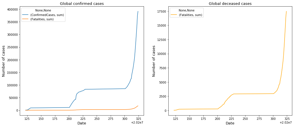
In order to find variable correlation to make sure that cases and deaths were worth pursuing I graphed it out. I took my training data set and graphed the global confirmed cases and the global confirmed deaths.
testData = pd.read_csv('test.csv')
trainData = pd.read_csv('train.csv')
display(trainData.tail())
| Id | Province/State | Country/Region | Lat | Long | Date | ConfirmedCases | Fatalities | |
|---|---|---|---|---|---|---|---|---|
| 17887 | 26378 | NaN | Zambia | -15.4167 | 28.2833 | 2020-03-20 | 2.0 | 0.0 |
| 17888 | 26379 | NaN | Zambia | -15.4167 | 28.2833 | 2020-03-21 | 2.0 | 0.0 |
| 17889 | 26380 | NaN | Zambia | -15.4167 | 28.2833 | 2020-03-22 | 3.0 | 0.0 |
| 17890 | 26381 | NaN | Zambia | -15.4167 | 28.2833 | 2020-03-23 | 3.0 | 0.0 |
| 17891 | 26382 | NaN | Zambia | -15.4167 | 28.2833 | 2020-03-24 | 3.0 | 0.0 |
display(testData.head())
| ForecastId | Province/State | Country/Region | Lat | Long | Date | |
|---|---|---|---|---|---|---|
| 0 | 1 | NaN | Afghanistan | 33.0 | 65.0 | 2020-03-12 |
| 1 | 2 | NaN | Afghanistan | 33.0 | 65.0 | 2020-03-13 |
| 2 | 3 | NaN | Afghanistan | 33.0 | 65.0 | 2020-03-14 |
| 3 | 4 | NaN | Afghanistan | 33.0 | 65.0 | 2020-03-15 |
| 4 | 5 | NaN | Afghanistan | 33.0 | 65.0 | 2020-03-16 |
The data I will be collecting will have to be well labeled and up to date. I looked for a couple different parameters. The only variables that I was curious in was; location, data, cases, deaths. With these variables I will be able to feed my model and make sure that I was answering my problem statement.
In order to make some observations I need to format the data to be useable and integers for graphing. The date field will be transformed into an integer by removing all symbols and setting the type as an int. Also, I will remove the NAN’s from the training set as those will provide no value. At the same time I will drop the Province/State column as I want to focus on the Country as a whole and not just individual states.
For the test data I want to make sure that I have the same primary key so I will use the date field and simply perform the same transformed as I did to the training dataset.
# Format date
trainData["Date"] = trainData["Date"].apply(lambda x: x.replace("-",""))
trainData["Date"]  = trainData["Date"].astype(int)

testData["Date"] = testData["Date"].apply(lambda x: x.replace("-",""))
testData["Date"]  = testData["Date"].astype(int)
# drop nan's
trainData = trainData.drop(['Province/State'],axis=1)
trainData = trainData.dropna()
trainData.isnull().sum()
Id                0
Country/Region    0
Lat               0
Long              0
Date              0
ConfirmedCases    0
Fatalities        0
dtype: int64
testData.isnull().sum()
ForecastId           0
Province/State    6622
Country/Region       0
Lat                  0
Long                 0
Date                 0
dtype: int64
trainData.nunique()
Id                17892
Country/Region      163
Lat                 272
Long                276
Date                 63
ConfirmedCases     1023
Fatalities          204
dtype: int64
testData.nunique()
ForecastId        12212
Province/State      128
Country/Region      163
Lat                 272
Long                276
Date                 43
dtype: int64
confirmed_total_date = trainData.groupby(['Date']).agg({'ConfirmedCases':['sum']})
fatalities_total_date = trainData.groupby(['Date']).agg({'Fatalities':['sum']})
total_date = confirmed_total_date.join(fatalities_total_date)

fig, (ax1, ax2) = plt.subplots(1, 2, figsize=(17,7))
total_date.plot(ax=ax1)
ax1.set_title("Global confirmed cases", size=13)
ax1.set_ylabel("Number of cases", size=13)
ax1.set_xlabel("Date", size=13)
fatalities_total_date.plot(ax=ax2, color='orange')
ax2.set_title("Global deceased cases", size=13)
ax2.set_ylabel("Number of cases", size=13)
ax2.set_xlabel("Date", size=13)
Text(0.5, 0, 'Date')
Observations
The only concern that is transparent here is that initially the graph starts out on a straight unaffected line. This could be due to the fact that in the wake of the new virus the healthcare industry was unsure of the true classification of the virus. This in turn will result in false readings and overlooked cases. When I focus my efforts on the United States I will start the data when the virus was recognized as an issue.Some issues that I see that could be affecting the graph would be the availability of the tests for the COVID-19 virus. Looking at the confirmed cases we can notice that the graph exponentially grew around the same time that the tests were distributed to the affected areas. This could affect the model.
matplotlib.style.use('ggplot')
plt.scatter(confirmed_total_date, fatalities_total_date)
plt.show()
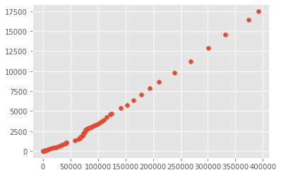
I used the scipy library to map out the correlations between the confirmed cases and confirmed deaths. When I used the spearman correlation I received a score of 1, then when I used the kendall tau correlation i got a score of .99. These scores show that there is a correlation between these two variables that when the confirmed cases goes up as does the deaths. But as I mentioned above this could also be reflective of when tests are being administered as that is when they become available in bulk. Or this could be reflective of the lack of response when first faced with the virus.
scipy.stats.spearmanr(confirmed_total_date, fatalities_total_date)[0]
1.0
scipy.stats.kendalltau(confirmed_total_date, fatalities_total_date)[0]
0.9999999999999999
United States Analysis
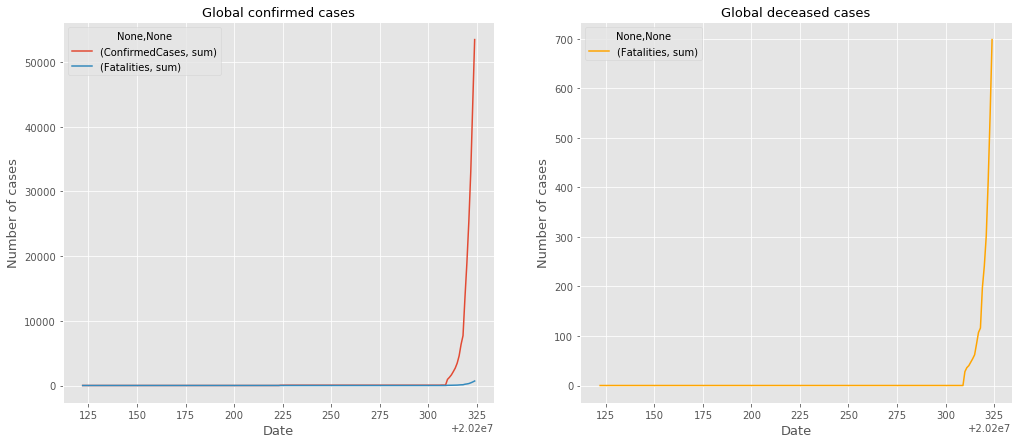
I want to identify all of the United States data in the datasets to identify a cleaner look. Once the Corona Virus became transparent in the United States there were tests available to test and identify for the virus. I anticipate that this analysis will differ from the rest of the world, graph above, as the graph will not include China. China’s influence in the data showed a delay in progression against the virus when it comes to tests and identification portrayed by the spikes in the data.
When the data comes to the United States I expect for it to start out slow then begin to grow exponentially as more tests will be available towards the beginning of the outbreak. China was unaware of the virus at first and allowed for the virus to spread. As the United States looking in, they should be able to catch the virus early on and take measures early on to prevent a wide spread disease.
unitedStates =trainData[trainData['Country/Region']=='US']
unitedStates.describe()
| Id | Lat | Long | Date | ConfirmedCases | Fatalities | |
|---|---|---|---|---|---|---|
| count | 3654.000000 | 3654.000000 | 3654.000000 | 3.654000e+03 | 3654.000000 | 3654.000000 |
| mean | 22584.500000 | 37.771567 | -84.323891 | 2.020024e+07 | 60.047072 | 0.813355 |
| std | 1557.201509 | 8.018508 | 46.996733 | 6.621358e+01 | 681.297097 | 7.030237 |
| min | 19903.000000 | 13.444300 | -157.498300 | 2.020012e+07 | 0.000000 | 0.000000 |
| 25% | 21236.250000 | 34.969700 | -99.784000 | 2.020021e+07 | 0.000000 | 0.000000 |
| 50% | 22584.500000 | 38.978600 | -87.944200 | 2.020022e+07 | 0.000000 | 0.000000 |
| 75% | 23932.750000 | 42.230200 | -76.802100 | 2.020031e+07 | 0.000000 | 0.000000 |
| max | 25266.000000 | 61.370700 | 144.793700 | 2.020032e+07 | 25681.000000 | 210.000000 |
confirmed_total_date_US = unitedStates.groupby(['Date']).agg({'ConfirmedCases':['sum']})
fatalities_total_date_US = unitedStates.groupby(['Date']).agg({'Fatalities':['sum']})
total_date_US = confirmed_total_date_US.join(fatalities_total_date_US)

fig, (ax1, ax2) = plt.subplots(1, 2, figsize=(17,7))
total_date_US.plot(ax=ax1)
ax1.set_title("Global confirmed cases", size=13)
ax1.set_ylabel("Number of cases", size=13)
ax1.set_xlabel("Date", size=13)
fatalities_total_date_US.plot(ax=ax2, color='orange')
ax2.set_title("Global deceased cases", size=13)
ax2.set_ylabel("Number of cases", size=13)
ax2.set_xlabel("Date", size=13)
Text(0.5, 0, 'Date')
Analysis
Taken from the same timeline we see that there was some time where the virus was not reported in the United States. But once the virus was reported we can see that the cases exploded.
The United States was aware of the virus as it originated in China. On Jan 21 2020 the United States had its first case of the virus. Then a month later Feb 26, 2020 the United States had it first suspected local transmission. Then a short three days later the United States had reported its first COVID-19 related death.
Looking at the graph above we notice that around early March there is a spike in the data. We are able to see that the graph started to grow. This is because on March 3, 2020 the CDC lifts restrictions for virus testing. This means that people will close contact with people diagnosed with COVID-19 or people with severe symptoms could get tested.
This, much like what had happened in China, availability in tests to the general public made it clear that the virus had already spread across the population. Once the testing was presented to the United States and people began to take the tests the volume of the virus came into light. Through the month of march the number of cases grew at an alarming rate because the availability of the tests gave us a clearer picture.
I expect this number to keep on growing as a result that tests are not accessible to everyone. Once there are enough tests to completely test everyone who is concerned with having the virus I expect the data to reflect a steady growth in cases and deaths.
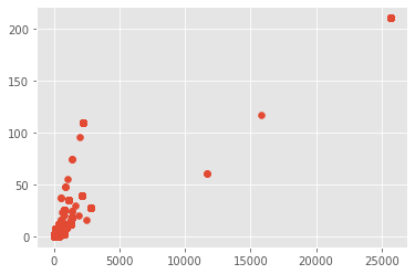
matplotlib.style.use('ggplot')
plt.scatter(confirmed_total_date_US, fatalities_total_date_US)
plt.show()
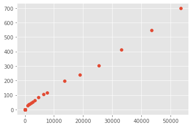
scipy.stats.spearmanr(confirmed_total_date_US, fatalities_total_date_US)[0]
0.8073991628275585
scipy.stats.kendalltau(confirmed_total_date_US, fatalities_total_date_US)[0]
0.7657375167529012
Correlation
When using the United States data the correlation scores between the confirmed deaths and confirmed cases got a spearman score of .80 and a kendall tau of .76. Even though this is not as strong as the global correlation there is still a correlation between the confirmed number of cases and fatalities in the United States. Even though the numbers are not similar, they follow a similar pattern and if the number of cases grow so with the number of deaths.
Random Forest Classification Model
The random forest classification model is an ensemble tree-based learning algorithm. The method is to randomly select a subset of training sets and it will aggregate the votes from different decision trees. This will allow the model to predict the final class of the test object.
The algorithm is stable and will not move or produce significantly different results if a new data set is introduced. The algorithm also does not have any bias. The algorithm can handle missing values and unscaled data points but for this project I have removed those concerns as it should lead to a better result.
from sklearn.ensemble import RandomForestClassifier
Tree_model = RandomForestClassifier(max_depth=200, random_state=0)
total_date_US
| ConfirmedCases | Fatalities | |
|---|---|---|
| sum | sum | |
| Date | ||
| 20200122 | 0.0 | 0.0 |
| 20200123 | 0.0 | 0.0 |
| 20200124 | 0.0 | 0.0 |
| 20200125 | 0.0 | 0.0 |
| 20200126 | 0.0 | 0.0 |
| ... | ... | ... |
| 20200320 | 18967.0 | 241.0 |
| 20200321 | 25347.0 | 302.0 |
| 20200322 | 33083.0 | 413.0 |
| 20200323 | 43442.0 | 547.0 |
| 20200324 | 53490.0 | 698.0 |
63 rows × 2 columns
train_unitedStates=unitedStates.drop(['Country/Region'],axis=1)
trainData_US=train_unitedStates[['Lat','Long','Date']]
trainData_US
| Lat | Long | Date | |
|---|---|---|---|
| 13482 | 32.3182 | -86.9023 | 20200122 |
| 13483 | 32.3182 | -86.9023 | 20200123 |
| 13484 | 32.3182 | -86.9023 | 20200124 |
| 13485 | 32.3182 | -86.9023 | 20200125 |
| 13486 | 32.3182 | -86.9023 | 20200126 |
| ... | ... | ... | ... |
| 17131 | 42.7560 | -107.3025 | 20200320 |
| 17132 | 42.7560 | -107.3025 | 20200321 |
| 17133 | 42.7560 | -107.3025 | 20200322 |
| 17134 | 42.7560 | -107.3025 | 20200323 |
| 17135 | 42.7560 | -107.3025 | 20200324 |
3654 rows × 3 columns
train_unitedStates.to_csv('unitedstatesdata.csv')
test_unitedStates =testData[testData['Country/Region']=='US']
test_unitedStates=test_unitedStates.drop(['Country/Region'],axis=1)
testData_US = test_unitedStates[['Lat','Long','Date']]
testData_US
| Lat | Long | Date | |
|---|---|---|---|
| 9202 | 32.3182 | -86.9023 | 20200312 |
| 9203 | 32.3182 | -86.9023 | 20200313 |
| 9204 | 32.3182 | -86.9023 | 20200314 |
| 9205 | 32.3182 | -86.9023 | 20200315 |
| 9206 | 32.3182 | -86.9023 | 20200316 |
| ... | ... | ... | ... |
| 11691 | 42.7560 | -107.3025 | 20200419 |
| 11692 | 42.7560 | -107.3025 | 20200420 |
| 11693 | 42.7560 | -107.3025 | 20200421 |
| 11694 | 42.7560 | -107.3025 | 20200422 |
| 11695 | 42.7560 | -107.3025 | 20200423 |
2494 rows × 3 columns
testData_US.tail()
| Lat | Long | Date | |
|---|---|---|---|
| 11691 | 42.756 | -107.3025 | 20200419 |
| 11692 | 42.756 | -107.3025 | 20200420 |
| 11693 | 42.756 | -107.3025 | 20200421 |
| 11694 | 42.756 | -107.3025 | 20200422 |
| 11695 | 42.756 | -107.3025 | 20200423 |
train_unitedStates_Confirmed=train_unitedStates[['ConfirmedCases']]
train_unitedStates_Confirmed.describe()
| ConfirmedCases | |
|---|---|
| count | 3654.000000 |
| mean | 60.047072 |
| std | 681.297097 |
| min | 0.000000 |
| 25% | 0.000000 |
| 50% | 0.000000 |
| 75% | 0.000000 |
| max | 25681.000000 |
train_unitedStates_Fatalities=train_unitedStates[['Fatalities']]
train_unitedStates_Fatalities.describe()
| Fatalities | |
|---|---|
| count | 3654.000000 |
| mean | 0.813355 |
| std | 7.030237 |
| min | 0.000000 |
| 25% | 0.000000 |
| 50% | 0.000000 |
| 75% | 0.000000 |
| max | 210.000000 |
x = trainData_US
y1 = train_unitedStates_Confirmed
y2 = train_unitedStates_Fatalities
x_test = testData_US
Tree_model.fit(x,y1)
predConfirmed = Tree_model.predict(x_test)
predConfirmed = pd.DataFrame(predConfirmed)
predConfirmed.columns = ["ConfirmedCases_prediction"]
/opt/conda/lib/python3.7/site-packages/ipykernel_launcher.py:1: DataConversionWarning: A column-vector y was passed when a 1d array was expected. Please change the shape of y to (n_samples,), for example using ravel().
  """Entry point for launching an IPython kernel.
predConfirmed
| ConfirmedCases_prediction | |
|---|---|
| 0 | 0.0 |
| 1 | 0.0 |
| 2 | 6.0 |
| 3 | 12.0 |
| 4 | 12.0 |
| ... | ... |
| 2489 | 29.0 |
| 2490 | 29.0 |
| 2491 | 29.0 |
| 2492 | 29.0 |
| 2493 | 29.0 |
2494 rows × 1 columns
Tree_model.fit(x,y2)
predFatalities = Tree_model.predict(x_test)
predFatalities = pd.DataFrame(predFatalities)
predFatalities.columns = ["Fatalities_prediction"]
/opt/conda/lib/python3.7/site-packages/ipykernel_launcher.py:1: DataConversionWarning: A column-vector y was passed when a 1d array was expected. Please change the shape of y to (n_samples,), for example using ravel().
  """Entry point for launching an IPython kernel.
predFatalities
| Fatalities_prediction | |
|---|---|
| 0 | 0.0 |
| 1 | 0.0 |
| 2 | 0.0 |
| 3 | 0.0 |
| 4 | 0.0 |
| ... | ... |
| 2489 | 0.0 |
| 2490 | 0.0 |
| 2491 | 0.0 |
| 2492 | 0.0 |
| 2493 | 0.0 |
2494 rows × 1 columns
predictions = predConfirmed.join(predFatalities)
predictions
| ConfirmedCases_prediction | Fatalities_prediction | |
|---|---|---|
| 0 | 0.0 | 0.0 |
| 1 | 0.0 | 0.0 |
| 2 | 6.0 | 0.0 |
| 3 | 12.0 | 0.0 |
| 4 | 12.0 | 0.0 |
| ... | ... | ... |
| 2489 | 29.0 | 0.0 |
| 2490 | 29.0 | 0.0 |
| 2491 | 29.0 | 0.0 |
| 2492 | 29.0 | 0.0 |
| 2493 | 29.0 | 0.0 |
2494 rows × 2 columns
fig, (ax1, ax2) = plt.subplots(1, 2, figsize=(17,7))
predictions.plot(ax=ax1)
ax1.set_title("US confirmed cases", size=13)
ax1.set_ylabel("Number of cases", size=13)
ax1.set_xlabel("Date", size=13)
predFatalities.plot(ax=ax2, color='orange')
ax2.set_title("US deceased cases", size=13)
ax2.set_ylabel("Number of cases", size=13)
ax2.set_xlabel("Date", size=13)
Text(0.5, 0, 'Date')

predictions.describe()
| ConfirmedCases_prediction | Fatalities_prediction | |
|---|---|---|
| count | 2494.000000 | 2494.000000 |
| mean | 690.180834 | 8.576183 |
| std | 2943.759642 | 27.336496 |
| min | 0.000000 | 0.000000 |
| 25% | 30.000000 | 0.000000 |
| 50% | 105.000000 | 1.000000 |
| 75% | 368.000000 | 6.000000 |
| max | 25681.000000 | 210.000000 |
matplotlib.style.use('ggplot')
plt.scatter(predConfirmed, predFatalities)
plt.show()
scipy.stats.spearmanr(predConfirmed, predFatalities)[0]
0.8056651838655811
scipy.stats.kendalltau(predConfirmed, predFatalities)[0]
0.6666551009677553
confirmedCasesPrint = predictions.sum()[0]
fatalititiesPrint = predictions.sum()[1]
print('By 4/23/2020 the below predictions were made: ')
print('{} more people in the US will contract the disease.'.format(confirmedCasesPrint))
print('As a result I predict that {} people will expire.'.format(fatalititiesPrint))
By 4/23/2020 the below predictions were made:
1721311.0 more people in the US will contract the disease.
As a result I predict that 21389.0 people will expire.
Conclusion
Upon using this model I was able to predict the following metrics. By 4/23/2020 the below predictions were made: 1,721,311.0 more people in the US will contract the disease, and as a result I predict that 21,389.0 people will expire. Between these numbers the correlation score was .80 for spearman and .66 for kendall tau. For this score I see a pattern that these numbers could represent valid numbers. Given the timeline with the skyrocketing numbers and the correlations of the predicted number I feel confident in the prediction.
Disclaimer
This project and data had been directly affected by the distribution of tests across the global. In the data and graphs we are able to see the spikes of which the tests became available based on location. In the United States we are able to see when tests are available and when supplies begin to deplete. I also suspect that those spike affected my outcome and the model of which I trained using that data. I suspect that the correlations between the two variables are accurate even if the numbers may be off.
Youtube Video link
https://youtu.be/Vg55Ry7Q7VU
Link to paper
https://github.com/SudoZyphr/covid19/blob/master/Covid-19.pdf
Resources:
- https://www.cdc.gov/coronavirus/2019-ncov/cases-updates/summary.html
- https://ourworldindata.org/coronavirus
- https://www.who.int/emergencies/diseases/novel-coronavirus-2019
- https://www.worldometers.info/coronavirus/
- https://informationisbeautiful.net/visualizations/covid-19-coronavirus-infographic-datapack/
- https://www.ecdc.europa.eu/en/publications-data/rapid-risk-assessment-novel-coronavirus- disease-2019-covid-19-pandemic-increased
- https://www.barrons.com/articles/latest-coronavirus-data-show-disease-continues-to-spread-even-in- the-u-s-51584224660
- https://www.theguardian.com/world/2020/mar/13/coronavirus-pandemic-visualising-the-global-crisis
- https://ourworldindata.org/coronavirus-source-data
- https://www.kaggle.com/sudalairajkumar/novel-corona-virus-2019-dataset
- https://www.sciencedaily.com/releases/2020/03/200317175442.htm
- https://www.worldometers.info/coronavirus/coronavirus-age-sex-demographics/